HTTM Part 5: It's an Oceanomenon!

It's time to face the final boss, Madden-Julian Oscillation

Apr 07, 2025

Pop artist Chappell Roan, who songs “Super Graphic Ultra Modern Girl,” “HOT TO GO!” and “Femininomenon” (read: feminine phenomenon) topped the charts last summer.

It always used to confuse me when someone would be called ‘an artist’s artist’ or ‘a writer’s writer.’ I thought it was obvious why writers wrote and painters painted: to commune with their fellow creatives as part of larger movements like Modernism or Impressionism. It was only recently that I realized this moniker was almost an insult: being a ‘writer’s writer’ meant your work is too niche to be appreciated by the general public. Famous for being brilliant yet inscrutable, such people use inventive yet obscure styles that can only be understood by those who are of the same mind — some oft-cited examples are Gertrude Stein, James Joyce and Cormac McCarthy. If you read and understand their works, you become part of a literary in-crowd, rendering you much cooler than anyone else in the world (as I and my fellow literature lovers can testify).

This is not to be confused with being your favorite writer’s favorite writer. That term is for those who have achieved widespread popularity. Being the favorite of a favorite automatically raises one’s stature — for example, last summer the singer Chappell Roan famously described herself as “your favorite artist’s favorite artist,” a quip that referred to both her drag queen idol and the boundless support she was receiving after making her big break. Because of her newfound fame, Roan had finally gotten the recognition other singers knew she deserved. She became a leader in the fields of pop music and drag culture, and even if you do not like her music it is impossible to ignore her influence (and Grammy win!).

But is it possible to be both an artist’s artist and a favorite’s favorite? The answer, as you will see with the Madden-Julian Oscillation, is yes! We close out the Hot Tub Time Machine series this week by examining something with particular relevance to both the scientific community and those of us who value our oceans and climate.

Recycling our knowledge

Before learning anything new, let’s dip our toes back in the hot tub and review what the time machine has revealed to us so far. To reiterate the metaphor, our ocean is like a giant hot tub that is slowly increasing in temperature. If we observe how certain phenomena change with the climate, we can predict how the ocean will move and change in the future. The main drivers of these small-scale climatic changes are known as climate oscillations, and they are born from air-sea interactions caused mainly by temperature changes. Water has a high specific heat capacity, meaning it takes longer to absorb heat than the air and holds onto it for longer periods of time. In each of the five previous installments of HTTM, we discussed…

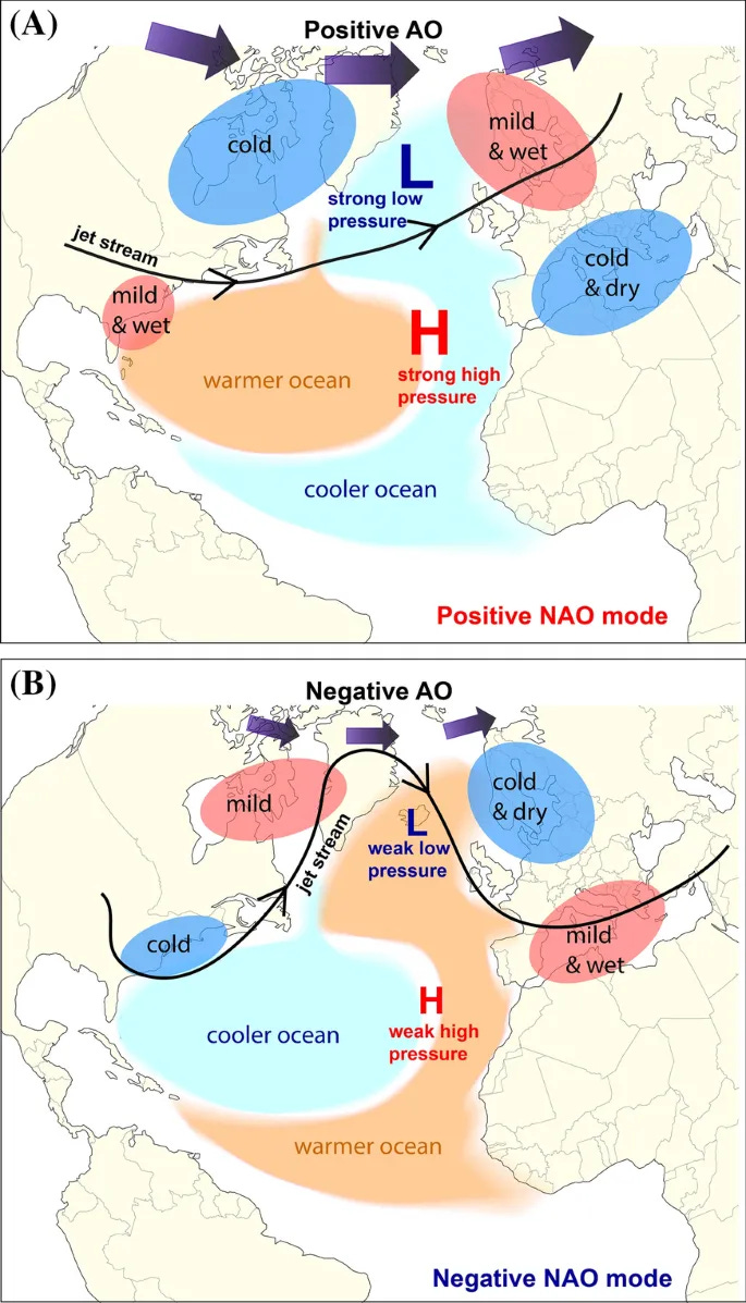
The North Atlantic Oscillation (NAO), which describes the atmospheric pressure differential between the Azores High and the Icelandic Low. The high creates mild, sunny conditions in the North Atlantic and the low creates windy, cool conditions over Iceland. It is mainly an atmospheric phenomenon and brings either excess moisture or excess heat to northern Europe during its positive and negative phases, respectively. It also affects weather in the Mediterranean (see graphic below).

The Atlantic Multidecadal Oscillation (AMO) is a measurement of the Atlantic Ocean’s heat content. It oscillates between positive (warmer than normal) and negative (cooler than normal) phases, which take upwards of 60 years to complete. This oscillation has a profound effect on the NAO as well as our global climate, influencing rainfall in the Sahel region of Africa and the severity of storms in North America, India and East Asia. This is because warmer waters leads to stronger storms: the more a parcel of water is heated, the likelier it will evaporate. The AMO has also been linked to short-term changes in ocean currents, according to a study published just last year.

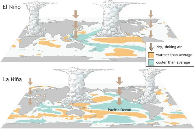
While the AMO and NAO may be new terminology, most people have heard of El Niño (government name the El Niño Southern Oscillation aka ENSO). ENSO is a large-scale pattern of both sea surface temperatures and atmospheric pressure, driven mostly by the changing strength of equatorial winds. Strong surface winds move water from the eastern edge of the Pacific to the western, creating a large area of stormy warmth around Southeast Asia. This causes cold, nutritious water from the Antarctic to upwell off the coast of South America, creating the dynamic known as La Niña. When surface winds are weaker, the warm sea water remains in the central and eastern Pacific, bringing large amounts of moisture and intensifying storms across the Americas, which we know to be an El Niño.

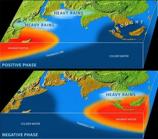
The Indian Ocean Dipole (IOD) is like a smaller version of ENSO: it too involves alternating locations of high & low pressure and cool & warm water, but it occurs in the Indian not Pacific Ocean. Its positive phase brings heavy rains to India and East Africa and is often blamed for particularly intense monsoon seasons (see graphic below). ENSO and IOD have been proven to work in tandem, feeding off of each other’s strengths and diminishing any weaknesses. Unlike ENSO phenomena, which happen over a period of 12 months, the IOD takes only 6 months to complete, meaning it can cause both mild winters and extremely hot summers in the span of one year!

Both the Arctic Oscillation (AO) and Antarctic Oscillation (AAO) are characterized by a natural fluctuation in air pressure in the upper latitudes. Such changes in pressure are caused by the amount of heat each pole can absorb. When the AO is positive, it brings light winds and mild weather to northern Europe and North America and drought to the Mediterranean; when it’s negative, the same areas as well as parts of Asia experience cold and stormy winters. The AAO affects weather in the Southern Hemisphere in a similar fashion, bringing mild weather to South America and Australia during its positive phase and deep freezes during the negative phase. While the AO and AAO do not affect the weather within the Arctic and Antarctica, they are so named because their mode is entirely dependent on the amount of heat reflected or absorbed by those poles.
Lastly, the Pacific Decadal Oscillation (PDO) describes long-term patterns of water temperatures north of the Equator. This oscillation controls where in the ocean warmer-than-average water can be found, and it works in tandem with the South Pacific Oscillation (SPO). Both oscillations either augment or diminish sea surface temperature anomalies in different parts of the Pacific. Since the SPO was only recently ‘discovered,’ there are very few scientific studies examining the scale of its influence.

Although some of these phenomena take place in overlapping areas of the ocean, only one has a truly global influence.

H-O-T-T-O-M-J-O

The Madden-Julian Oscillation (MJO) was first discovered in 1971 by meteorologists named (you guessed it) Madden and Julian. These two men analyzed 10 years of data from Kanton Island in what is now Kiribati and found consistent, original patterns of increasing air temperatures and wind speeds that occurred every 41-53 days. Unlike all the previous phenomena we covered, which oscillate like a see-saw in one part of the world, the MJO travels across the equator as fast as 18mph (8 m/s)! After a low pressure cell develops on the east coast of Africa, it then travels eastward across the equator until reaching the Americas, where it usually — but not always — dissipates. To fuel its movement, it sucks air in from the east, creating a large area of high pressure that acts as a butler, announcing imminent extreme rainfall in India, Southeast Asia, Oceania and sometimes as far as North & Central America.

The MJO is similar to all other oscillations because it too has a dipole structure: one half has high atmospheric pressure and low sea surface temperatures (negative/suppressed phase), and the other half has low atmospheric pressure and high sea surface temps (positive/convective phase). One can detect the MJO by observing when a pair of high and low pressure areas are moving eastward across the equator at a consistent pace. As it propagates, it brings intense heat to the ocean waters and excess moisture to the atmosphere; on the back end of the phenomenon, waters are left cooler and calmer than normal. The distance it travels is proportional to how fast it’s moving, which can vary depending on the time of year as well as any localized changes in climate it encounters.

In this Australia-centric diagram, you can see the moisture cell of the Madden-Julian Oscillation traveling from the eastern Indian to central Pacific Oceans.

Since there can be multiple iterations of the MJO per season, scientists are able to observe the oscillation’s effects on specific weather phenomena. For example, a research paper about the devastating 2019 cyclone Fani, which made landfall on India state of Odisha on May 3^rd of that year, discovered that MJO had made it possible for a cyclone to form closer to the equator than usual. This meant that the storm had access to large amounts of warm water and was able to maintain its strength as it crossed the Indian Ocean because the MJO was guiding its path (Singh et. al.). The timing of the MJO, however, is very important: a 2021 study by Balaguru et. al. found that the MJO’s negative phase reduced sea surface temperatures by as much as .47°C (0.85°F), which led to a 50% reduction in the intensity of cyclones.

#InfluencerStatus

Only recently have scientists begun to publish research proving the MJO’s effects on other climate phenomena. For example, oceanographers in the Indian Ocean found that higher-than-normal sea surface temperatures, which are influenced by the IOD, can independently trigger the MJO. Similarly, in 2017 scientists determined that North Atlantic Oscillatory events last for a longer periods of time when the Madden-Julian Oscillation is active, but when the MJO is negative, NAO phases only lasted for 10 days at a time. This is because the NAO relies on strong winds to carry atmospheric moisture to its part of the globe, and the MJO’s positive/convective phase is known to increase wind strength. This is especially noticeable after the MJO makes its way to the eastern Pacific, where powerful winds in the upper atmosphere carry its remnants across North America into the North Atlantic.

It also should come as no surprise that the Madden-Julian Oscillation works as an ENSO-enhancer. A 2018 study by Godoi et.al., based on decades of research, found that when the suppressed/negative phase of the MJO moved over the western Pacific during a La Niña, there were a larger number of abnormally-high waves. The same phenomenon was observed when the convective/positive phase of the MJO passed over the same spot where an El Niño was occurring. Wave height is a good measure of energy transfer from the atmosphere to the ocean (similar to how evaporation transfers energy in the opposite direction). The faster or most consistently surface-level winds blow, the higher ocean waves become and the more energy they carry with them as they crash into coral reefs, atolls, and barrier beaches. Godoi et.al. concluded their results “highlight the need to assess atmospheric and oceanic conditions considering multiple climate oscillations.”

“But what we really need is a(n Oceanomenon)”

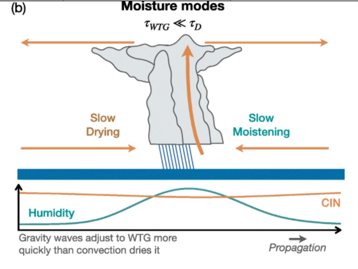
As with all climate oscillations, there is currently a debate about whether it generates from atmospheric or oceanic conditions. In this ‘chicken-or-the-egg’ (or should I say ‘air-or-the-sea’) scenario of what causes an MJO to develop, changes in sea surface temperatures almost always anticipate the formation of low pressure cells in the atmosphere. A leading theory about this phenomenon is called the Moisture Mode Theory. Proposed in 2001 by Raymond et. al., it states that the strength of MJO phases and their propagation across oceans are directly affected by “large-scale horizontal and vertical moisture advection, which moistens the free troposphere to the east of the MJO convection center and dries to the west.” In other words, these scientists believe heat transfers from the surface ocean to clouds in the atmosphere and back again, creating an insular cell which is then moved eastward across the globe by the system’s search for new pockets of warm water.

What this graphic from Adames et. al. 2021 explains is that the warmth transported to the upper atmosphere by evaporation *strengthens* gravity’s pull on the MJO, resulting in it being pulled along the equator.

The air-sea interactions which form the building blocks of climate phenomena are hugely important to climate models. Such predictive graphics are increasingly relied upon by research labs and the private sector alike to predict our uncertain future. Because scientists are continually searching for ways to improve their models, there are endless papers published on modeling strategies and mishaps. This ‘meta-climatology,’ as I like to call it, has unearthed evidence of models’ systematic dismissal of the sea’s influence. After a 2015 research paper criticized MJO models for “offer[ing] limited insight on the role of ocean feedbacks,” several other studies published in the past decade blamed incorrect prediction on the modelers’ failure to take evaporation into account. I am stating the obvious when noting how ninety percent (90%) of our atmosphere’s water comes from oceans and other bodies of water, and these climatologists were making trying to predict a phenomena that travels across not one but two major oceans! So by diminishing the importance of evaporation, these models effectively deleted the ocean from the equation. As a separate research group observed quite brilliantly “the inclusion of air-sea interaction can lead to significant improvement in simulating the MJO.”

Conclusion: Super Graphic Ultra-Modern Oscillation Like Me

Clearly, computers and scientists alike are creating less-accurate climate models because of their inability or unwillingness to consider the ocean. But as the fields of computer science and climatology continue to expand and overlap, including complex ocean dynamics in models has never been easier. In 2018 an atmospheric researcher at Yale University wrote about the abundance of evidence suggesting “the MJO is becoming stronger as the oceans warm.” He proved his theories by using a different type of climate model than most scientists use. Lagrangian atmospheric models take into account each parcel of water as unique, which is different from the standard Eulerian model, which examines the flow of water, not the water itself. Both types of models have been around for decades, but the Lagrangian is slowly becoming more popular because it can more easily account for variability.

Although breaking down our entire air-sea system into little tiny parts can be tedious, doing so allows one to account for the complexities of climate change. The ocean is no longer a constant in these equations, and continuing to treat it as such reduces the accuracy of our predictions. In their original paper, Madden and Julian worried that a “lunar-tidal frequency” had affected their data, showing they too understood the profound effect oceans can have on our atmosphere. Until climate models account for the ocean’s role in oscillations like the MJO, they will continue to yield less-reliable predictions.

In Circulation

Discussion about this post